PART 4
At last - the derivation of the equation
And what this tells us
 Note that there are two small equal sided right angle triangles:
 One with two equal sides of length I%,
and
One with two equal sides of length D%.
Hence by adding up the vertical distances we can see that:
P% = C% + D% + I%
WHAT THIS TELLS US
This means that ALL debt repayment schedules have these three parts, whether intentionally or not. There is no debt repayments schedule which has no value of e% or no value of P%. Since all debt repayment schedules have a value P% they also have a value for C%, D%, and I%.
Even if e% = 0% as with Level Payments, the location of the 'X' that describes the repayments is on this chart and so P% contains a value for D% and a value for C% and a value for I%.
LOOKING FOR SAFE MORTGAGES
/ OTHER DEBT STRUCTURES
Given that D% needs to be positive, we can decide which debt repayments models are safe and which are not. Those that have no control over D% are not safe - at least not for people. A government can mange with D% = 0% without getting payments fatigue because tax revenues go on and on and should never depart too far from AEG% p.a. even in a recession.
Since the value of D% is the distance of the 'X' from the AEG% p.a. line, it follows that if e% = 0%, as it is with a fixed interest mortgage or a fixed interest government bond, then since the AEG% p.a. line is always on the move, the value of D% p.a. is always on the move. In fact, AEG% p.a. can go negative as it has done in some European countries recently.
The effect on this of I% can be very nasty. Remember:
I% = r% - AEG% - (iii)
For example, if r% = 3% nominal interest
AEG% = -5% p.a.
You get I% = 8% p.a.
That is 8% of the income borrowed added to the debt by the true rate of interest. A debt of 4 times income then rises at 4 x 8% = 32% of income p.a.

The mortgage schedule begins to look like this:
This also affects an investment in a government bond hugely during a slow down or a recession. Below is a graph showing how that has affected the return on US treasuries on a year by year basis since 1980 when inflation was high and since when it has fallen to almost zero. The effect is the same:
Try r% = 20% and then AEG% falls from 25% to 11%. You get I% = 20% - 25% at first = -5%
But then this becomes
I% = 20% - 11% as inflation comes down = 9%.
This is like what happened to USA Government Bonds and the result was this graph:
 |
| Source: Morgan Stanley Research c/o Money Game Chart of the day. Figures adjusted by Edward for AEG to reveal the true rates of return. |
As can be seen the return on USA AAA rated bonds reached 25% one year and averaged something like the trend-line shown. This average reflects the cost to USA tax payers of using fixed interest bonds over that period.
This additional GDP added to the total government debt is probably enough compounded up to explain most of the rise in USA government debt since that time! For example, 5% p.a. compounded over 25 years comes to a 3.6 fold increase in the original number of GDP owed in 1980 if no repayments were made. Certainly 9% true interest would not have been paid. Some part of it maybe would. Even paying 5% is steep.
THE DANGER OF A BOND CRISIS
Now that interest rates are virtually zero there is a significant danger that the value of these bonds may collapse when Quantitative easing is reduced and interest rates rise. This can produce another world crisis of enormous proportions and is the worry of one Andy Haldane at the Bank of England as expressed in The Guardian newspaper recently (before this weekend of 15th June 2013). His remarks may be enough to cause another panic - we will see.
The interest rate sensitivity of mortgage finance is also very great and it is this which accounts for the rise and fall of property prices and which can also undermine the whole economy.
In both cases we need to reform the debt structures.
IN SUMMARY
The cost-to-income of the fixed interest mortgages or even the low interest rate mortgages rises every year if average incomes are falling. The same applies to government fixed interest rate debt / bonds. The cost rises every year. This is not safe, and it leaves investors not knowing what kind of I% they will get on their investments. If a recovery comes then I% can even go negative. So this arrangement is not safe for borrowers or for investors / lenders.
Given the amount of wealth invested in both housing and government bond sectors this is very distressing to the performance of the whole economy.
What we are looking for is a repayments model which looks something like the sketch already presented twice now:
Repayments follow a more 'normal' rental type model, rising with incomes but not quite as fast.
Looking at the equation:
P% = C% + D% + I%
we see that adding in D% to get this slope adds to the value of P% - the initial cost of the repayments.
Putting D% p.a. = 4% adds 4% to P%.

Such a repayments model might look like this if I% had been fixed at 3%. (I% can be fixed by offering fixed true rate wealth bonds to investors).
The downwards slope means that D% p.a. is positive. In this illustration the payments start at 30% of income and reduce at 4% p.a. to reach around 11% at the end of 25 years. The slope is the value of D% and so it is based on the AEG% p.a. index of incomes, not individual incomes. But if the slope is steep enough all borrowers within reason should be able to cope with the repayments.
In practice the straight sloping line should be curved, but it helps to make the point when I do not show the curves of compounding.
As already pointed out there is a BIG problem with Level Payments and Fixed Interest
Let's do a short revision course.Originally I wrote the following script about the fixed interest mortgage model - it goes over what I just wrote above, but in a different way:
Given that, by definition:
D% = AEG% - e% - (ii)
we can see that fixing e% = 0% can lead to problems when AEG% is close to zero because if e% = 0% for level fixed payments and AEG% = 0%, then D% = 0%.
Example for austerity:
AEG% = -2% and e% = 0% gives:
D% = - 2% - 0% = -2%
So as already mentioned above, the payments are costing a 2% higher proportion of average income every year. Like this:

Here D% p.a. is negative so the slope is up instead of down and payments are rising relative to average income every year.
What is worse is that the value of I% also rises. I% governs the cost-to-income that the borrower has to repay. I% adds wealth to the wealth debt already owed. Suppose that the lender offered a fixed rate of nominal interest with r% = 3% but then AEG% fell to -2%. We know that:
I% = r% - AEG% - (ii)
So I% = 3% - (-2%) = 5%.
This is more costly to the borrower than raising equity capital. For lenders 5% above AEG% p.a. pays better than investing in equities and property. I am assuming the equities investment data on that for the USA / UK applies here.
For other nations lenders need to do more researches to reach their figures. But normally one would expect a high rate of return that out-performs long term investments in equities and property to lead to major problems for prospective new borrowers and a flood of money on the books of lenders which they would not be able to lend.
As already noted, normally the value of I% (net of lending costs and taxation) should not exceed the rate of return on such other investments but it should also be above zero to limit the demand for borrowing.
PREVENTING THE NEXT CRISIS
Imagine that a UK lender was to offer a 10 year fixed true interest rate of 5% p.a. The number of older people wanting a safe investment that performed that well would be very high. It would provide a very safe annuity. I have listed a whole range of uses for this kind of bond on this page called NEW FINANCIAL PRODUCTS RESULTING.
As soon as these kinds of wealth bonds become available there will be a major clamour for such products because nothing sells better than risk free (to wealth) investments. But to make that happen in time to prevent Andy Haldane's feared crisis there needs to be a commission of enquiry set up and an IMPLEMENTATION programme developed as outlined on that same blog.
There we are discussing the replacement of fixed interest bonds with wealth bonds in a very different environment of low true interest rates - but safe wealth will attract a massive demand at an rate of true interest in the environment that currently prevails. Doing so will safeguard the banks' balance sheets. Offering the replacement wealth bonds at a discounted price would cut the government's debt.
Investors face the alternative of imploding bond values as interest rates rise, so a discounted rate may well be popular.
Going back now to looking at the upper boundary for I% in more normal economies:
The number of borrowers wanting to borrow at a 5% level of I% would be much fewer because the slope for D% p.a. would reduce to 2% p.a. compared to the illustration above:
P% = C% (about the same) + D% (2% less = 2%) + I% (2% more).
By keeping C% the same the total repayment period would remain close to 25 years. To do that D% has to drop to compensate for the higher level of I%.
Then we get this:

The slope is 2% less and the total cost is a lot more.
I will come back to this a bit later with more detail.
CONCLUSIONS
1. A fixed interest mortgage does not look viable when AEG% p.a. is falling. For another example if AEG% = 10% and r% = 13% fixed, what happens when AEG% p.a. falls to 5%?
I% = 3% at first but then rises to 8%.
This is similar to what happened to the USA government bonds in the 1980s. See above. It meant that AAA rated bonds were yielding far more than share investments ever did over the longer term.
2. If we look at the main equation:
P% = C% + D% + I%
We can see that a rising level of I% requires a lower value of D% if P% and C% and the total repayment term are to remain the same.
In fact if I% increases by 1% the D% must decrease by 1% or the mortgage will go off schedule as C% adjusts instead. Or P% will rise - taking us back to the same old problems that we are having with variable interest rate mortgages now.
For the moment let us not look at variable rates. Above we are looking at fixed true rates. So if the fixed true rate on offer to lenders out there in the market for say 10 year bonds or longer, rises by 1% then D% will fall by 1%.
SUMMARY SO FAR AND MORE
I named the main equation P% = C% + D% + I%
Ingram's Safe Entry Cost Equation because it can be used for setting the entry cost (the initial value of P%) and because I was unable to patent it I attached my own name to it.
Interestingly the value of P% does not depend upon the value of either r% or AEG%. It depends on I% which is the difference - the marginal rate at which wealth gets added to the debt.
I% = r% - AEG%
So the rate of inflation, or AEG% p.a., in a nation should not affect the amount that can be lent safely - by much.
The most important difference would be the variability of incomes growth between different members of the working population. If this gets too big then it needs a larger D% to accommodate it.
In fact this is a general equation which can be applied at any time to any form of regular payment debt. It takes the basic elements of Payments Depreciation, D% p.a. Capital repayments C% p.a., and wealth addition (I% p.a.) and adds them together to get the cost of the payments P% p.a.
P% = C% + D% + I% - all are p.a. - (i)
PART 5
A DETAILED LOOK AT TRUE INTEREST I%
AND WEALTH
First, some more revision...REMEMBER:
I% is not the nominal rate of interest 'r%'; it is the marginal rate above AEG% p.a. I called this the True rate of interest.
I% = r% - AEG% - (ii)
ABOUT TRUE INTEREST I%
When the interest rate = AEG%, say 4% p.a. and incomes are rising at the same 4% p.a. the amount owed at the end of the year is 104 per 100 debt.
But if incomes also rose by 4% the debt / income ratio is no higher:
If income was 100 at the start of the year it will also be 104 by the end of the year.
So a year's income was borrowed and even without making any repayments at all, the loan will still be one year's income at the end of the year.
Only the excess interest above AEG% p.a. increases that ratio. Only that excess (marginal / true) interest adds to the cost of borrowing for a person on average income increases.
If r% = 10% then the loan will be 110 at the end of the year and if incomes are rising by only 4% p.a. then income will be 6% less at 104.
I% = 6%
At this rate the income owed increases by 6% p.a. compared to the income borrowed. But we are talking here of average incomes...
BORROWERS V INVESTORS
New script
What the borrower sees and what the investor / lender sees are not the same.
We can think of borrowers as not all getting average income increases. For those with incomes growing less quickly the cost-to-income will be higher. For those with incomes growing more quickly the cost-to-income will be lower.
For the investor looking to lend money and to preserve the years of income that has been saved and lent, they want to keep pace with, or do better than, the average / the index, much as they may expect to do over the long term with equities or property. All have a loose link to AEG% p.a. the aggregate demand baseline of economies.
However, market forces, or counter-inflation policy, will determine the interest rate unless it has been distorted by something.
DEFINING WEALTH
So let us define wealth as the number of years' income that has been lent.
This definition of wealth is useful because when I% is positive it moves wealth from the 'average borrower' to the investor. In this sense, wealth can be defined in units of National Average Earnings, NAE.
NAE is the part of the national income that a person has earned as income or profits, or has been given, or acquired in some way.
If that part of National Income is not preserved when it is invested, some other person or entity will spend the part that has been lost.
For example, look at this spreadsheet which is produced by the EXCEL sheet mentioned earlier as being for sale:
FIG XX - Negative true interest moves wealth from lender to borrower
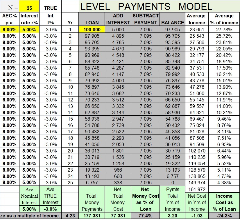
This income (wealth) has not been lost. The borrower first spent the income (NAE) that he/she borrowed / was lent, and then repaid less NAE so he/she was able to spend the income / wealth (NAE) saved on something else. The table does not show the NAE but one could try this: assume that the borrower was on average income and then the table does show NAE. 4.23 NAE was borrowed and 3.20 NAE was repaid.
Wealth did not vanish - it moved. 1.03 NAE moved from the lender to the borrower.
The same applies if I% is positive - wealth moves but this time in the other direction.
TAX DISTORTION
If we look at the MONEY repaid in the above illustration it looks like a 77.4% profit. That gets taxed - haha! Some joke. Some distortion.
Distortions all cost the economy and the social fabric something, so we will need to look into this and see how we can sort it out without messing anything up. It can be done.
In America they give tax relief on the interest paid! Giving tax relief on AEG% of the interest is a variable rate gift and another distortion. It is not needed. The net result of both tax regimes combined (taxation of all interest and tax relief on all interest), is to tax saved wealth and give it to borrowers. It reduces the ability of lenders to keep interest rates down. The main effect is to increase administration costs.
In reality, in the above scenario (see the table again), the borrower spends the 4.23 years' income right away and only has to repay 3.2 years' income leaving him/her free to spend the remainder at will on whatever is wished.
A year's spending power has left the lender and moved to the borrower.
Imagine if the borrower's property has risen at the same rate as AEG% p.a. That is quite possible, even probable. He/she will do very well.
He/she borrows at AEG% - 3% p.a. and his property rises in value at AEG% p.a. and attracts rental on top.
TRUE COST DEFINED
If I% is positive, we now can see that the cost-to-wealth of the repayments, as opposed to the cost-to-income of a particular borrower, is the true cost (actual cost to wealth). The true cost is not the cost to the income of a particular borrower. It is the wealth that has been borrowed plus the overall cost of the marginal interest rate I% which has increased the wealth owed and added to the wealth of the lender.
TWO MEASUREMENTS
In all my spreadsheets readers will find two cost figures:
There is the money cost and
There is the wealth cost, or the 'true cost' as I call it. This is the number of year's income that it takes to repay if the borrower's income rises as fast as average. True cost can also be expressed in NAE. For governments it can be expressed as a fraction or a percent of GDP.
The two figures, money cost and true cost usually look very different.
When inflation is high and interest rates are high the cost to money can be very high indeed, yet at the same time the cost to income can be very low or even negative.
This means that the figures offered to the public can be very misleading.
REAL INTEREST IS NOT ENOUGH
Even if the figures are adjusted for prices inflation they can be very misleading:

Here the nominal interest rate is 12% and prices inflation is 7% so the real interest rate is 5%:
12% - 7% = 5% real interest.
But the true interest rate is only 2%:
12% - 10% (AEG%) = 2%
If the nominal interest rate had been 8% then the real interest rate would have been +1%:
8% - 7% inflation = +1% real interest
but the true interest rate (I%) would have been -2%
8% - 10%(AEG%) = -2%
8% interest means that a loan of 100 becomes 108 at year's end
But incomes would be 110 by year's end.
So now we see that the average borrower will not need to repay the whole year's income that was borrowed. 2% less wealth will need to be repaid than was borrowed just in that one year. Yet the real rate of interest was +1%. Real interest does not protect wealth.
So an index-linked investment which is linked to prices does not protect wealth.
You do NOT find that in your text books!
MISSING TABLE
I compiled a table to show how much 'wealth profit' an investor can get from buying a fixed true rate bond at various rates of interest and I included the cost to a borrower over a 25 year term from borrowing at the same rates of interest. I will add this table when I locate it. I gave an example of 5% true interest increasing wealth by 3.6 fold though. So it can be seen that quite small amounts of true interest are very attractive to older people seeking security.
THAT EUREKA THING
NOW we see why it was so important to introduce I% into the main equation. I% is the rate of wealth transfer. A high I% is a serious factor in any debt repayments schedule. Wealth as measured / added by I% is a real and tangible thing that has never been declared in our text books.
And it brings to the fore the importance of AEG% as a baseline for everything in the economy - all forms of investment are propelled by AEG% p.a. - by aggregate demand and how fast it changes.
If we adjust all prices and repayment costs for AEG% p.a. everything will be seen as if there was no AEG% p.a. Everything is relative to AEG% p.a. Only the excess I% adds a cost or a benefit. Only I% moves wealth.
SUMMARY
True interest is a key component of the economy. It is responsible for wealth transfer on a massive scale, even when it is not very high.
The text books are not telling it as it is when they write of real interest rates. Real interest rates do not preserve wealth.
A true rate of interest of zero incorporates the real rate of economic growth (approximately) and is a great selling point to raise funds for lenders - and for governments. Yet it costs the borrowing house buyer or government no actual wealth.
Eureka! - What have we been thinking all this time?
PART 6
TESTING APPLICATIONS OF THE EQUATION
The data that I have for the UK shows that the true interest averaged +3% on home loans from 1970 to 2002. I got a similar figure for South Africa and I used this 3% figure to forecast by how much the Fed might need to raise interest rates in 2006 / 8. My forecast was almost exactly in line with what was actually targeted. It was just that to target such a 4.5% raise in interest rates implied a 58% increase in the cost of variable rate prime mortgage payments!
I wrote this page on Finding the Mid-Cycle Rate of Interest as a result of that calculation / observation.
Clearly, you cannot lend a whole lot more just because, temporarily, interest rates have fallen, no matter how far they have fallen.
So I have used 3% true interest as a baseline for my studies and simulations - the assumed average rate. Readers can experiment with other average rates and I have done that too. My spreadsheets are available for sale. So given that baseline:
Given that P% = C% + D% + I%
We can put in some figures:
P% = 1.5% + 4% + 3% = 8.5% p.a.
This is approximately the data that represents a 25 year mortgage repaid with 4% p.a. Payments Depreciation and at 3% true interest.
It creates a mortgage of 3.5 times income.
This is the original 3.5 times income mortgage that I illustrated above where the payments fell at 4% p.a. and which cost 30% of income falling to around 11% of income (shaded area) when I% = 3%.
If the true interest rate I% is 5% this means that D% now has to reduce D% from 4% p.a. to 2% p.a. because I% is 2% higher:
P% = 1.5% + 2% + 5% = 8.5% as before - so we still have a 3.5 times income mortgage because the entry cost is still the same.
We cannot reduce C% because that will cause the loan to take longer to repay.We do not want to increase P%, because that will hit collateral security / house prices, (but we can lean that way), so what is left is D%. This value must fall by 2% if I% rises by 2% as shown in this sketch.
Tests show that if the current true rate of interest is +11% or -7% (two extreme figures taken from South African data), the entry cost can still be set close to this mid-cycle figure because such extremes reverse and go the opposite way. The true rate still averages about the same figure.
I will add some back-testing data on a new page when I have time. It is already there for customers on the spreadsheet.
I want to move this next PART to be the next item before I go to red font above.
PART 7
From here on readers will find extracts from the earlier paper which is still to be found on the next blog page - MATHS 1
The Risk Management Chart and the standing loan line also works when e% is negative and payments are falling.
FIG 1.4 – Payments falling - but with the 'X' above the standing loan line, the debt is falling faster than the payments. If the 'X' was on the standing loan line both the payments 'P' and the loan 'L' would be falling at the same pace. But neither of them would reach zero. Ever.

So here, at the tip of the arrow, the standing loan line shows that the payments are falling (e% = -4% p.a say), but the payments are so high that the loan size is also falling by 4% p.a. Neither 'L' nor 'P' ever reach zero. Every year 96% of what was there the previous year remains as the balance owed at the end of the current year.
When we place the ‘X’ above the standing loan line as shown and with AEG% p.a. = 0% as shown in FIG 1.4, with r% = 3%, the loan will fall faster than the payments and the mortgage will be repaid on schedule. See FIG 1.5 below.
When we place the ‘X’ above the standing loan line as shown and with AEG% p.a. = 0% as shown in FIG 1.4, with r% = 3%, the loan will fall faster than the payments and the mortgage will be repaid on schedule. See FIG 1.5 below.
FIG 1.5 – Payments Falling with e% = -4% p.a. and AEG% p.a. = 0% (Average incomes not rising). D% = AEG% = 4% p.a.

The good news is that in this case, with incomes not rising, it is likely that the economy is in recession, and / or the rate of interest is very low. So the standing loan line is much lower as shown in FIG 1.5. But to achieve this level of D%, P% may be almost the same 8.5% p.a. as before the recession.
SIZE OF MORTGAGE
At this level of P% = 8.5%, the amount that can be lent on 30% of income in repayments is 3.5 years' income. You can use gross income or net income as long as you use the same figure for both. Lenders decide how much of the gross income should be affordable and whether or not 30% is the right figure.
TOTAL COST TO INCOME
If you add up all of the '% of incomes' you get the total cost-to-income of the repayments which is shown as 4.8 years' income, or 1.25 years' income more than was borrowed, which is 35.2% more than was borrowed as shown.
If we put P% = 8.5% when AEG% p.a. = 4% and the true interest rate is still 3% as in the above example, the amount lent will still be 3.5 years' income and the repayments will cost 34.9% more than the income borrowed, (almost the same figure).
A true interest rate of 3% is the long term average rate of true interest (my estimate) for the UK. Notice that the amount lent in both of these examples is 3.5 years' income. As stated earlier, the value of P% does not depend on the nominal rate of interest. It is a function of the true rate of interest I%:
P% = C% + D% + I%
COMMENT
Did you know that the IMF's Country Report 2012 said that house prices are now averaging 4.5 years' income whereas long term in the UK they have averaged 3.5 years' income? That was when 3.5 years' income mortgages were common. Now, with interest rates being held very low, they are lending more but they are not making enough provision for interest rates to rise. See FIG 1.6
This should follow an illustration of the Hybrid ILS mortgage.
I will insert that.
The risk management chart is very similar. It is a simpler thing to illustrate before we get to this one.
HAZARD OF ECONOMIC RECOVERY
FIG 1.6 - Look where the lower 'X' is placed. Note how when interest rates rise the standing loan line will rise forcing the 'X' to jump up the Y-Axis adding over 30% (maybe 50%) to the entry cost of new mortgages and hitting both property prices and variable rate mortgages hard.
The AEG% p.a. line will move to the right.

To avoid or postpone this problem is why keeping interest rates down is essential to economic recovery - so they say. If they allow interest rates to rise naturally, the cost of borrowing will jump sky high and property values will drop. The banks will be threatened again, not just by property prices tumbling and arrears and repossessions rising, but also their reserves invested in fixed interest bonds will also take a beating. But they have not seen this chart and the solution to the problem which is to move the 'X' to the right. And they have not read the next page on government bonds.
When the 'X' gets moved to the right as a rescue operation for the Level Payments Model, this is known as the ILS HYBRID Mortgage Model. It starts as a Level Payments Model but gets rescued by the ILS move to the right!.
When the 'X' gets moved to the right as a rescue operation for the Level Payments Model, this is known as the ILS HYBRID Mortgage Model. It starts as a Level Payments Model but gets rescued by the ILS move to the right!.
If you would like to use the spreadsheets that I use to produce all of these illustrations, including a full range of bar charts and spreadsheets, and the ability to input historic data as you wish, you may buy a copy. This is really the only way to thoroughly understand the subject and to test the proposed debt models. Send me an email to:
The cost to a full time student is very low. The cost to an institution is high - you may not share the software with others. One copy per computer.
GENERAL APPLICATION
OTHER MORTGAGE MODELS
In order to convert from one style of debt repayment model to another you just need to change the way in which you are managing the values C% and D%.
EXAMPLES If r% and P are both index-linked to a prices or an incomes index then you have a problem. You are not managing D%.
If the payments are linked to the wages index as in Turkey, then D% = 0%.
If payments are linked to prices then D% is approximately the rate of real economic growth, which can turn negative.
Most index-linked models (all that I know of) index-link both the payments P (e% p.a.) as well as the interest rate r%. As stated, this means a loss of control over D%. In fact, the only models that mange D% appropriately are these ILS Models, based on this mathematics.
THE SAFEST MORTGAGE OF ALL
Sorry - this is a bit repetitive but sometimes repetition helps...
There is one ILS Model in which I% is fixed by agreement with the lender / investors who also get a fixed I% p.a. reduced by costs. In such a case, as the lender adjusts the value of r% as AEG% varies so as to keep I% constant.
I% = r% - AEG% = constant
This gives a very safe:
P% = C% + fixed D% + fixed I% - remember that P% and C% are not fixed: every year as capital is repaid they both increase by the about the same small (at first) %.
Eventually they both exceed 100% and the small remaining debt is paid off.
This is fixed I% Defined Cost Mortgage is VERY safe because D% is fixed no matter what is happening to r% or AEG%. The fixed I% provides the lender with a positive and guaranteed return on wealth which can be passed on to the savers / investors. There is little risk of arrears because D% is fixed.
DODGING BASEL III issues
A lender can even find investors and match them to individual borrowers, taking no risk themselves. Or lenders can set up a unit trust (Mutual Fund) for deposits and lend those funds, again without taking any risk themselves. The lender is then just an agency of the unit trust fund.
-----------------------------
Legal frameworks willing, any mortgage can be converted to any other kind of mortgage at any time.
P% = C% + D% + I%
The difference is just a matter of how, and if, the values on the right hand side are managed.
-------------------------------------
The rest I may change - or delete.
What is mostly missing is a LOT of illustrations with spreadsheets. These are fascinating.
I will put them on a new blog page.
What is mostly missing is a LOT of illustrations with spreadsheets. These are fascinating.
I will put them on a new blog page.
Next Session
MANAGING THE ARREARS RISK
Now we are going to look at variable rate ILS Mortgages. Variable rates can be cheaper because they tend to be funded by 'hot' money that is in the form of short term, fast access deposits upon which little or no interest is paid.
If interest is paid then rates adjust to changing conditions and the 'market rate' is established. When one has a fixed rate, the market rate can go higher or lower and this presents a 'market rate risk' to the fixed rate investor - the risk of being out of line and losing out as a result. For this reason investors like to add a bit of interest to be on the safe side of that risk.
With variable rates, however, the lending / borrowing risk of payments getting out of control depends upon how high the value of C% and D% are at outset and what is likely to happen to the value of I% over time.
Remember the equation:
P% = C% + D% + I%
If I% is constant then over time the outstanding repayment period shortens every year because the ratio P/L rises - the loan reduces and the payments P remain the same. This means that C% rises and P% rises every year if the mortgage is to be repaid on time.
P% = P / L x 100%
But if I% is not a constant then, unless some adjustment is made to D%, that rising P% and C% pattern gets disturbed.
One could re-write the equation this way:
P% = F% + I%
where F% = C% + D%.
So if I% rises then F% has to fall to keep P% on course.
But in practice we would not want to disturb C% on its steady upwards path, needed to keep the repayment term on schedule. The shorter the remaining years to pay, N, the higher the value of C% has to climb. So that leaves us with a falling F% when I% rises but only the D% part of F% may be allowed to fall:
This means that in a perfect world, D% has to be large enough to stay positive when I% rises.
HOW TO SET THE SAFE ENTRY COST
SETTING I% FOR VARIABLE INTEREST RATES
The key to creating a safe variable rate mortgage, or even a safe fixed true interest rate mortgage, lies in managing D%. For this reason, the initial value of I% used to calculate a safe value for P% will not be the current value of I%.
We can modify my Safe Entry Cost Equation:
P% = C% + D% + (I% + K%)
We will not use the current value of I%, but instead we will add K% to that - K% being the amount needed to increase or reduce the current value of I% so as to make it approximately equal to the median value of I% over a cycle.
In other words, I% + K% = the median value of I%. The reason for this follows below.
NOTE ON MEDIAN VALUE
It may be better to call this 'median' value the clearing value of I%. That is the value which applies to mortgage finance when the cost of borrowing / the cost of money in the economy is such as to hold inflation steady. Aggregate demand for money is comprised of numerous arrangements from overdrafts through business loans and mortgages to government debt. The median value is the value of interest rates at which the overall demand for money is not leading to an inflationary increase in the supply of money / credit.
There is no clear way to define this figure so I have simply taken a few studies of past rates and concluded that for the developed economies it is close to 3% for mortgage finance, this being the average true rate over long periods before rates were distorted downwards at the start of this century.
The back testing done (to be added to later pages) seems to show that this method of finding the entry cost P% is workable for variable rate mortgages. In the event of a mistake being made the worst that will happen is that P% has to be raised or the repayment period extended, which is what we were trying to avoid because that is the problem we have currently with variable rate mortgages.
In practice, with the way that so many things are currently distorting interest rates we know that I% can be down at -7% or up at +11%.
But we also know that the further it departs from the median value or the value that should balance the supply of funds to lend with the demand for them, which appears to be around 3% for the UK for example, the faster it will return to the median value and probably overshoot in the opposite direction.
But we also know that the further it departs from the median value or the value that should balance the supply of funds to lend with the demand for them, which appears to be around 3% for the UK for example, the faster it will return to the median value and probably overshoot in the opposite direction.
Past data shows that this is not a big worry for lenders. They can smooth this volatility out by not adjusting D% proportionately, but instead allowing the projected value of N to fluctuate around the target value as C% rises and falls, C% even going negative at times.
Alternatively, lenders can observe that a one year spike of 11% in I% would take D% to -7% (say) making the cost of repayments rise by 7% more than incomes are rising. This is less than the worst case result for a Level Payments Mortgage after a 1% interest rate increase. So it would not be a big problem. The following year it may swing back to I% = - 6% so then D% switches to +10% making payments fall by 10% relative to incomes. As a trend, the falls in the payments are always bigger then the rises.
Alternatively, lenders can observe that a one year spike of 11% in I% would take D% to -7% (say) making the cost of repayments rise by 7% more than incomes are rising. This is less than the worst case result for a Level Payments Mortgage after a 1% interest rate increase. So it would not be a big problem. The following year it may swing back to I% = - 6% so then D% switches to +10% making payments fall by 10% relative to incomes. As a trend, the falls in the payments are always bigger then the rises.
ESTIMATING THE MAXIMUM I%
The best way to set the Safe Entry cost appears to be to set it by estimating the maximum sustainable value of I% for the economy and the lending industry concerned. It is likely that this maximum value is likely to be less than the true rate of return (above AEG%) on other investments which are more risky.
For UK and USA Equities this may be less than say 5% p.a. true (above AEG% p.a.) and less than that for property, but the detailed studies of past data seem to show that the sustainable value of I% has to be positive above AEG% p.a. by around 2% or more to prevent inflation from running out of control.
For UK and USA Equities this may be less than say 5% p.a. true (above AEG% p.a.) and less than that for property, but the detailed studies of past data seem to show that the sustainable value of I% has to be positive above AEG% p.a. by around 2% or more to prevent inflation from running out of control.
This does not mean that 'Sustainable I%' or the Median value if 'I%' will stay within those narrow limits, between about 2% and 4% for the UK. It does mean that it will not deviate far for very long. Tests show that short term deviations from mean, even large ones, can be accommodated as just outlined and as readers will see in the illustrations to be given in the later pages (writing in progress).
As already stated, the worst that can happen is that P% and so P, the current monthly payments, may have to make some upwards adjustment, if I% moves above the anticipated range and stays there, just as happens with the current variable rate Level Payments (LP) mortgage model, but more likely current ILS mortgages will be allowed to extend their repayment period and new mortgages will cost more.
As already stated, the worst that can happen is that P% and so P, the current monthly payments, may have to make some upwards adjustment, if I% moves above the anticipated range and stays there, just as happens with the current variable rate Level Payments (LP) mortgage model, but more likely current ILS mortgages will be allowed to extend their repayment period and new mortgages will cost more.
SETTING D%
Setting D% is another issue. Consider how volatile income increases are so that D% is large enough to cope with that. More volatile pay rises means that there will be a larger variation (standard deviation maybe) among individuals' wage increases, requiring D% to be increased so as to cope with the laggards.
The critical value for D%, the value when too many borrowers will be unable to cope, (too many may be 5% or more - it is a matter of culture, politics, and opinion), needs local researches to be done to see how far adrift - how far behind the average - an individual borrower's income may lag behind the index selected. See the page on Defining the index for more on that.
The critical value for D%, the value when too many borrowers will be unable to cope, (too many may be 5% or more - it is a matter of culture, politics, and opinion), needs local researches to be done to see how far adrift - how far behind the average - an individual borrower's income may lag behind the index selected. See the page on Defining the index for more on that.
As mentioned earlier, we want to leave C% alone when I% increases so that the mortgage is repaid on time. So the value of D% will take the strain. If we use too low a value for I% when we set the entry cost value of P% (the first year value), then as I% rises to its maximum sustainable level, D% will fall too low to be comfortable.
Either the value of P% will have to jump up as it does with the current variable interest rate mortgages, or there will be payments fatigue and there will be arrears. And probably the new entry cost for new mortgages will be high and property values will fall endangering collateral security, besides re-distributing wealth among the population.
Either the value of P% will have to jump up as it does with the current variable interest rate mortgages, or there will be payments fatigue and there will be arrears. And probably the new entry cost for new mortgages will be high and property values will fall endangering collateral security, besides re-distributing wealth among the population.
For most economies that are reasonably stable, the initial / entry cost value of P% based on these considerations ought to be reasonably stable because the median value of I% used in the entry cost calculation will also be stable. In the UK my opinion is that it would lie between 2% and 3% and stay there for decades unless something fundamental changes, possibly like the new regulations coming in that would raise lending costs, and a 4% value of D% mimics incomes rising at 4% p.a. (whether they are rising or falling), which looking at past records suggests a very low, almost invisible rate of arrears.
So in such a case,
P% = 1.5% or similar, + 4% (D%) + 3% (I% sustainable) = 8.5% and stable.
The mortgage multiple would be 3.5 years' income and stable, rising in a proportionate way as incomes rise. As mentioned earlier, the Country Report from the IMF in July 2012 stated that long term UK property prices had averaged 3.5 years' income. And in those days 100% mortgages were on offer.
MAJOR BREAKTHROUGH
This means that the amount of wealth (income multiple) lent and the cost of housing will rise with rising incomes / aggregate demand, which is what every other good and service and rentals may be expected to do, ceteris paribus.
THAT is a major breakthrough on its own. The whole spending and cost patterns in the economy can harmonize. Wealth gets safer and costs become easier to forecast.
It takes out a lot of arrears risk, collateral security risk, and wealth re-distribution for the community. It puts the construction industry onto a secure footing. It helps the whole economy to grow.
This means that the value of property used as collateral will not bubble and burst, but will remain sufficiently stable that a 100% mortgage may not be out of the question. Even more than 100% can be lent in some conditions based upon the presumption that a borrower does not wish to abandon his/her home and end up owing money as well. This depends on the law of the land supporting the lender, and the cultural attitude to debt.